Fulfilling Orders – An Algorithm Engineering Exercise

Recently, Zalando Software Engineering organized a hackathon on a website called hackerrank.com. The event was conveniently scheduled on a Saturday, and I decided to participate as I was curious. The problems that were to be solved in the hackathon were algorithmical, very well explained, and required to think about the nature of the problems in order to be solved correctly. All in all, taking part in the hackathon was a very nice experience, and I later used one of the problems as a challenge problem to exercise algorithm engineering with one of my PhD students. The problem is defined as follows:

Problem Definition:

We are organizing the shipping process in a company and have a set of orders on file. There are three different types of goods, let's name them , , and , and every customer can only order one item of every good type. So there are 7 different orders that a customer can make:

Ordering only an item of type
Ordering only an item of type
Ordering only an item of type
Ordering an item of type and one of type
Ordering an item of type and one of type
Ordering an item of type and one of type
Ordering items of types , , and .

Let us use the variable names , , to denote how many items of each type our company has in stock, and let us use , , , , , , and xyz as variable names for denoting how many orders of each of the above types we have.

We want to find a subset of the orders whose number (cardinality) is as high as possible such that fulfilling them all does not exceed the number of items in stock.

We can formalize the problem by asking for some number of fulfilled orders

such that

which state that there is a limited supply of each good type, and the constraints

which state that not more orders can be served than there are in the order book. All numbers are integer and non-negative.

Efficiency Requirements:

The solution (algorithm) should work with numbers in the 1000s and there is a computation time limit of 2 seconds (for solutions in C) or 10 seconds (for solutions in Python) on a moderately modern computer, so brute forcing all possible combinations of values , , , xy' , xz' , yz' , xyz' up to some sufficient bound (such as, e.g., max(X,Y,Z) ) is infeasible.

A First Lazy Solution: Integer Linear Programming

The problem definition above looks quite simple: We are given 10 integer constants (

) and we search for values for the integer variables

, and

that maximize x' + y' + z' + xy' + xz' + yz' + xyz'

. Since all constraints listed above are linear and the optimization function is linear, we can model this problem as an integer linear program (ILP).

ILP solving is a classical technique in operations research and nowadays, off-the-shelf solvers are available to solve so-called linear programs. The word “program” in this context refers to a set of constraints on the solution and an optimization function, so there is nothing to be programmed in the software-engineering sense. For 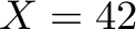X = 42

, such a linear program in the input format for the lp_solve tool looks as follows:

max: x+y+z+xy+xz+yz+xyz;

x<=5;
y<=7;
z<=18;
xy<=20;
xz<=20;
yz<=20;
xyz<=5;

x+xy+xz+xyz <= 42;
y+xy+yz+xyz <= 23;
z+xz+yz+xyz <= 51;

int x;
int y;
int z;
int xy;
int xz;
int yz;
int xyz;

Note that the dashes of the variables names have been left out in the input file as the undashed variables do not appear named in the problem instance file. The lp_solve tool easily computes a solution in less than 10 ms on a moderately modern computer. The output of the tool looks as follows:

Value of objective function: 66.00000000

Actual values of the variables:
x                               5
y                               7
z                              18
xy                              3
xz                             20
yz                              8
xyz                             5

Now we could say that we are done with solving the problem as the approach works reasonably fast, but using an ILP solver would defeat the purpose of the hackathon. So there should be a solution that is reasonably simple to implement using only language features and standard libraries of commonly used programming languages. It should also be noted that ILP solving is NP-complete, so there probably exists no fast algorithm for solving this problem. Since the number of variables and constraints is fixed, this is not a big concern, but the question remains if there is a more direct solution that also yields insights into the main properties of the problem. I expected this to be the case, as otherwise the problem would be an odd choice for a general-audience hackathon.

A First Analysis

Probably the first idea that comes into mind when trying to maximize the number of orders fulfilled is to execute them greedily. We order the variables

into a list and then iterate over the list. While doing so, we update

, and

by executing as many orders of the respective order types as possible and subtracting the number of items used for doing so from

and

Example:

Let us try out this idea on an example. We fix the order xyz , , , , , , for X = 42 , Y = 23 , Z=51 , x=5 , y=7 , z=10 , xy=15 , xz=20 , yz=20 , and xyz=5 . The following table represents the variable values while the algorithm tries to fulfill as many orders as possible:

text{ begin{tikzpicture} node[inner sep=4pt] (a) at (0,0) { begin{tabular}{l||l|l|l||l} textbf{Order type considered} & makemath{X} & makemath{Y} & makemath{Z} & textbf{Executed orders} hline hline - & 41 & 23 & 51 & - hline makemath{xyz} & 36 & 18 & 46 & makemath{xyz: 5} hline makemath{xy} & 21 & 3 & 46 & makemath{xy: 15} hline makemath{yz} & 21 & 0 & 43 & makemath{yz: 3} hline makemath{xz} & 1 & 0 & 23 & makemath{xz: 20} hline makemath{x} & 0 & 0 & 23 & makemath{x: 1} hline makemath{y} & 0 & 0 & 23 & makemath{y: 0} hline makemath{z} & 0 & 0 & 13 & makemath{z: 10} end{tabular} }; end{tikzpicture} }

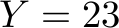
The overall number of orders fulfilled in this example is 54. But is it optimal? We try ordering the orders differently – this time, we just use the reverse order compared to the previous table.

This time, we computed a plan to serve 58 orders, which is more than before.

The example shows that when following the greedy approach, the order of the orders is important. But which one is the right one? Intuitively, larger orders should be processed last, as they drain the number of items in stock more than smaller orders, but both type of orders count in the same way towards the overall objective. This line of thought can be completed by considering (for the example case of

and

orders) that there is never a reason to prefer an

order over an

order – the latter requires a strictly smaller amount of resources, so whenever we have a solution for the fulfilled orders in which not all

orders are fulfilled and some

orders are fulfilled, then we can translate it to a solution in which one more

order is fulfilled at the cost of fulfilling fewer

orders. Similarly, the xyz

orders should only be fulfilled if the number of orders fulfilled of all other types has been maxed out, as fulfilling xyz

orders is strictly more expensive than fulfilling any other order. So the second order in the example above is not bad. The xyz

orders are checked last and the order of the first three order types does not matter, as the

and

orders are independent. The only thing that is not obvious is in which order to fulfill the

, and

orders.

Since there are only three different orders of {xy,xz,yz}

, it is quite simple to try out all orders of them. So we would run the greedy algorithm for the orders

and just pick the best possible solution that we find with any of these orders. If a greedy approach is correct, then one of them will yield the best solution.

Putting this idea into an algorithm implementation is quite simple, and for the said hackathon this is the solution that I submitted. The hackerrank.com website gave me full credit for the solution as it works correctly on all test cases on which it was checked. While I wasn't entirely sure whether the solution is really a good one, at the point, I moved on to the other problems in the competition, as it required me to be as fast as possible with solving all problems (and I was not done at that point). After the competition, I checked which solution the winner of the competition had (which seems to be possible if you submitted a solution getting you 100% of the points). It was essentially the same, except that it was written in C++ (while I wrote mine in Python).

After I gave this problem to my PhD student and he came with the same solution, I however requested him to prepare a correctness proof of this idea, as it is not at all obvious whether this solution is really correct. As it turns out, that is because it actually isn't correct.

A More Balanced Use of Resources

To see the problem with the approach above, let us consider an example with only two-item orders (as we have already found out that they are the ones for which a trade-off may need to be made).

Example:

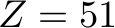
Let us have X = 18 , Y = 18 , Z=18 , x=0 , y=0 , z=0 , xy=18 , xz=18 , yz=18 , xyz=0 . Due to the symmetry of the example, we only need to consider one ordering of the order types, which, without loss of generality, we choose to be xy, xz,yz .

Using the algorithm from above, we thus fulfill all orders of one type and keep the others untouched. Overall, 18 orders are fulfilled. This is less than optimal, as we can also execute 9 orders of each type, which leads to an empty stock and 27 orders having been fulfilled.

So what still seems to be missing is the idea to balance the consumption of the items such that the greediness does not keep us from fulfilling later order types in the order type list. But when is that the case? An idea is to plan two order types greedily at a time. If for example for the

and

order types, we can fulfill

of such orders in total, we may want to balance these

orders between

and

types in a way that maximizes min(Y,Z)

afterwards, as this leaves as many resources for the

order type as possible. But we can still try to maximize xy + xz

first, as unnecessarily leaving an

item in stock cannot make a solution better.

Now how many orders of types

and

can we fulfill? We can fulfill at most min(Y,xy)

most orders of type

and at most min(Z,xz)

types of type

, and we can never fulfill more orders of types

and

together than

. Together, this gives us b = min(X,min(Y,xy)+min(Z,xz))

many orders of

and

. Now, we need to balance the ones of types

and

to be fulfilled. Let xy'

be the number of

orders fulfilled. We want to maximize

Choosing

such that

is the best way to maximize this expression (as

is constant), so we compute:

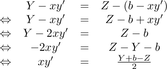
At the same time xy'

is bounded from below by

and from above by

, so

should be truncated accordingly when using the equation above. In case xy'

is non-integer, this means that after fulfilling the

and

orders, one of the numbers of remaining

and

items has to be odd. In this case, whether xy'

is rounded up or down should intuitively not matter, but we should verify this intuition somehow.

import sys
import math

# Read the input problem
(X,Y,Z) = [int(a) for a in sys.stdin.readline().strip().split(" ")]
nofOrders = int(sys.stdin.readline().strip())
orders = {(0,0,1):0,(0,1,0):0,(1,0,0):0,(0,1,1):0,(1,0,1):0,(1,1,0):0,(1,1,1):0}

for i in range(0,nofOrders):
    data = sys.stdin.readline().strip().split(",")
    thisTuple = [0,0,0]
    for a in data:
        if a=="A":
            thisTuple[0] += 1
        elif a=="B":
            thisTuple[1] += 1
        elif a=="C":
            thisTuple[2] += 1
        else:
            print("'"+a+"'")
            assert False
    orders[tuple(thisTuple)]+= 1

# Get the values into the variables
x = orders[(1,0,0)]
y = orders[(0,1,0)]
z = orders[(0,0,1)]
xy = orders[(1,1,0)]
xz = orders[(1,0,1)]
yz = orders[(0,1,1)]
xyz = orders[(1,1,1)]

# Serve single items
totalNofOrders = 0
totalNofOrders += min(X,x)
X -= min(X,x)
totalNofOrders += min(Y,y)
Y -= min(Y,y)
totalNofOrders += min(Z,z)
Z -= min(Z,z)

# Two-item orders
b = min(X,min(Y,xy)+min(Z,xz))
xyf = (Y + b - Z) // 2
xyf = max(0,min([xy,xyf,b]))
totalNofOrders += b
X -= xyf
Y -= xyf
X -= (b - xyf)
Z -= (b - xyf)
yzf = min(min(yz,Y),Z)
totalNofOrders += yzf
Y -= yzf
Z -= yzf

# Three-item orders
totalNofOrders += min([X,Y,Z,xyz])

# Print result
print(totalNofOrders)

The first couple of lines read the input problem in the format described on the hackerrank.com problem page. To simplify reading the code, they are then copied to variables with the same names as in the equations above. Then, the number of fulfillable orders is computed and the program prints out this number. In the original problem description on hackerrank.com, this was the only expected output, so the program does not do more than that. Note that the variable xyf represents the number of

orders fulfilled.

Funnily, this program only fulfills 14 of the 17 test cases on hackerrank.com. Looking at the example, we can see that the program prints higher numbers of fulfilled orders than expected. This is not surprising, as we possibly gave a strictly better solution than the one accepted by the website. But again we should verify that the program is really correct rather than assuming that because the test cases on hackerrank.com accept a sub-optimal solution, it is OK for our (hopefully) correct program not to satisfy all test cases.

So the main question is now if we found a correct solution. The explanation above gives some intuition on why one may believe this computation to be correct, but perhaps we are overlooking something? We could now prepare a formal mathematical proof (where we may still make some errors), but for this program, there is an easier way to check the solution for correctness.

Verifying the solution

The algorithmic main part of the program above is actually quite simple: it only performs a few basic calculations on the variables

, and

, and the program does not have any loops. The difficulty in program verification is typically to find suitable loop invariants, but since we do not have any in this example, we can use an SMT solver to check the program for correctness.

In an input instance to an SMT solver, we ask for a valuation of some variables such that certain requirements that we can express in a closed form are fulfilled. In this regard, SMT solving is similar to integer linear program (as we used above), but more flexible in what can be modeled. This flexibility comes at a computational price, but the use of the min

function makes it appear as if the added expressivity would be helpful. Why exactly this is the case is unfortunately beyond the scope of this document, so let us just assume that an SMT solver is a rational choice for verifying our solution.

But what is it that we are searching for? We want to see if there are some values for

, and

for which the program above computes a sub-optimal solution. A solution has this property if there is a better solution. Since in SMT solving, the variables can have all values that fulfill all constraints, we start by stating the properties that the other solution should have. Let us use the variables x_1

, and

to model the number of fulfilled orders in the optimal (or at least better) solution. We have the following constraints on them:

Now we need to define how the algorithm above behaves. As SMT instances model mathematical problems, there is no concept of reassignment for variables. Thus, whenever in the program a variable value is overwritten, we need to use a fresh variable to define the new value in the program from that point onwards. Let us use the variables x_2

, and

to model the number of fulfilled orders in the solution computed by the program above. We have the following constraints:

Finally, we need the constraint that the optimal solution is better than the one computed with the algorithm:

We can now build an SMT instance that captures all of these constraints. We refer to the Tutorial of the SMT solver Z3 for a description of the syntax of the input files, and move straight to the solution.

(declare-const x Int)
(declare-const y Int)
(declare-const z Int)
(declare-const xy Int)
(declare-const xz Int)
(declare-const yz Int)
(declare-const xyz Int)

(declare-const x1 Int)
(declare-const y1 Int)
(declare-const z1 Int)
(declare-const xy1 Int)
(declare-const xz1 Int)
(declare-const yz1 Int)
(declare-const xyz1 Int)

(declare-const x2 Int)
(declare-const y2 Int)
(declare-const z2 Int)
(declare-const xy2 Int)
(declare-const xz2 Int)
(declare-const yz2 Int)
(declare-const xyz2 Int)

(declare-const X Int)
(declare-const Y Int)
(declare-const Z Int)

(assert (>= x 0))
(assert (>= y 0))
(assert (>= z 0))
(assert (>= xy 0))
(assert (>= xz 0))
(assert (>= yz 0))
(assert (>= xyz 0))

(assert (>= x1 0))
(assert (>= y1 0))
(assert (>= z1 0))
(assert (>= xy1 0))
(assert (>= xz1 0))
(assert (>= yz1 0))
(assert (>= xyz1 0))

(assert (>= X 0))
(assert (>= Y 0))
(assert (>= Z 0))

(define-fun min2 ((a Int) (b Int)) Int (ite (< a b) a b))
(define-fun max2 ((a Int) (b Int)) Int (ite (> a b) a b))

(assert (<= (+ x1 xy1 xz1 xyz1) X))
(assert (<= (+ y1 xy1 yz1 xyz1) Y))
(assert (<= (+ z1 xz1 yz1 xyz1) Z))
(assert (<= x1 x))
(assert (<= y1 y))
(assert (<= z1 z))
(assert (<= xy1 xy))
(assert (<= xz1 xz))
(assert (<= yz1 yz))
(assert (<= xyz1 xyz))

(assert (= x2 (min2 X x)))
(declare-const X2 Int)
(assert (= X2 (- X x2)))

(assert (= y2 (min2 Y y)))
(declare-const Y2 Int)
(assert (= Y2 (- Y y2)))

(assert (= z2 (min2 Z z)))
(declare-const Z2 Int)
(assert (= Z2 (- Z z2)))

(declare-const b Int)
(assert (= b (min2 X2 (+ (min2 Y2 xy) (min2 Z2 xz)))))

(assert (= xy2 (max2 0 (min2 xy (min2 b (div (- (+ Y2 b) Z2) 2))))))

(assert (= xz2 (- b xy2)))
(declare-const X3 Int)
(assert (= X3 (- (- X2 xy2) xz2)))
(declare-const Y3 Int)
(assert (= Y3 (- Y2 xy2)))
(declare-const Z3 Int)
(assert (= Z3 (- Z2 xz2)))

(assert (= yz2 (min2 (min2 yz Y3) Z3)))
(declare-const Y4 Int)
(assert (= Y4 (- Y3 yz2)))
(declare-const Z4 Int)
(assert (= Z4 (- Z3 yz2)))

(assert (= xyz2 (min2 X3 (min2 Y4 (min2 Z4 xyz)))))

(assert (< (+ x2 y2 z2 xy2 xz2 yz2 xyz2) (+ x1 y1 z1 xy1 xz1 yz1 xyz1)))

(check-sat)

Most of the lines are concerned with declaring variables, ensuring that all variables whose values are not computed by our algorithm are all non-negative, and defining the behavior of the algorithm.

The SMT solver z3 by Microsoft Research returns quickly ( < 0.1

seconds on a moderately modern PC) that there is no assignment to the variables that satisfies all constraints. So unless a modeling error has been made, the program above never returns sub-optimal solutions.

Now that we know that the program does not miss optima, the question arises whether perhaps there is still another bug lurking somewhere in the code, e.g., because the algorithm returns incorrect solutions. We can use z3 again to find it. What we want to obtain is an input to the algorithm such that the solution is not correct. We already established correctness conditions for the reference solution in the SMT instance above, and modify the last assert statement of the instance to allow variable valuations for which either the solution computed by the algorithm above is suboptimal or incorrect. Since the correctness condition consists of many conjuncts, it suffices if just one of the is violated. We replace the last assert statement in the above code by:

(assert (or
    (< (+ x2 y2 z2 xy2 xz2 yz2 xyz2) (+ x1 y1 z1 xy1 xz1 yz1 xyz1))
    (< x2 0)
    (< y2 0)
    (< z2 0)
    (< xy2 0)
    (< xz2 0)
    (< yz2 0)
    (< xyz2 0)
    (> (+ x2 xy2 xz2 xyz2) X)
    (> (+ y2 xy2 yz2 xyz2) Y)
    (> (+ z2 xz2 yz2 xyz2) Z)
    (> x2 x)
    (> y2 y)
    (> z2 z)
    (> xy2 xy)
    (> xz2 xz)
    (> yz2 yz)
    (> xyz2 xyz)
))

This time, z3 computes a sat result, so there may be a case where the program behaves incorrectly. After adding the line (get-model) to the SMT instance and running z3 again, we obtain the following output:

sat
(model
  (define-fun X2 () Int
    4)
  (define-fun z1 () Int
    0)
  (define-fun xyz () Int
    0)
  (define-fun Y4 () Int
    1)
  (define-fun x2 () Int
    1)
  (define-fun xyz1 () Int
    0)
  (define-fun xy1 () Int
    3)
  (define-fun yz () Int
    1)
  (define-fun z2 () Int
    0)
  (define-fun Y () Int
    5)
  (define-fun xy2 () Int
    2)
  (define-fun xy () Int
    3)
  (define-fun yz2 () Int
    0)
  (define-fun z () Int
    0)
  (define-fun xz2 () Int
    2)
  (define-fun Y2 () Int
    3)
  (define-fun y2 () Int
    2)
  (define-fun y1 () Int
    0)
  (define-fun y () Int
    2)
  (define-fun xyz2 () Int
    0)
  (define-fun xz () Int
    1)
  (define-fun x1 () Int
    0)
  (define-fun yz1 () Int
    0)
  (define-fun xz1 () Int
    1)
  (define-fun X () Int
    5)
  (define-fun b () Int
    4)
  (define-fun Y3 () Int
    1)
  (define-fun Z () Int
    2)
  (define-fun X3 () Int
    0)
  (define-fun Z4 () Int
    0)
  (define-fun x () Int
    1)
  (define-fun Z2 () Int
    2)
  (define-fun Z3 () Int
    0)
)

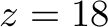
This output format is cumbersome to read, so let us rearrange it. The input to the algorithm is:

We can see that this is suboptimal as it leaves one-item orders unfulfilled even though there is enough stock to fulfill at least one more of them. The solution that – according to the SMT instance – our implementation generated is:

The problem seems to be that our implementation produces a solution in which more

orders are fulfilled than there are available. We need to distinguish the cases that the SMT instance was written down incorrectly and the case that the Python code above is actually wrong. So we generate the test case found by the SMT solver as an input to the Python program using the format described in the hackerrank.com problem description. It looks as follows:

5 5 2
8
A
B
B
A,B
A,B
A,B
A,C
B,C

Note that the last few lines represent the orders, and on the original problem page, the items are called A, B, and C rather than

, and

as we used as item names here. Running the program (with some additional code lines to output the numbers of fulfilled orders) shows that the program computes exactly the (non-)solution that the SMT solver found. So the program is indeed working incorrectly, and we actually found the bug using an SMT solver. Not bad at all.

Fixing the Bug

What seems to be the problem with the first version of the code is that variable

is not looked at when deciding how many orders of types

and

to fulfill. The number of

orders to fulfill is actually b - xy_2

in the equations above, so xy_2 = max(0,min(xy,b,lfloor (Y_2 + b - Z_2) / 2 rfloor))

should not be too low to make sense of this idea. We can see that the problem seems to be that we need xy_2

to be high enough to have xy_2 + xz_2 = b

. So we modify this equation to:

(assert (= xy2 (max2 0 (min2 xy (min2 b (div (- (+ Y2 b) Z2) 2))))))

(assert (= xy2 (max2 (- b xz) (max2 0 (min2 xy (min2 b (div (- (+ Y2 b) Z2) 2)))))))

Running Z3 again yields that there is indeed no model for this SMT instance (which you can download here). We only need to fix a single line in the Python code to incorporate this change. Running the program (which you can download here) on the test case above yields:

Finally, we want to see if the new program makes more test cases on hackerrank.com pass. After all, we have evidence that the SMT instance and the Python program coincide (as they both exhibited the same bug), and the result by the SMT solver suggests that the program is now correct. There can always be some more modeling errors in the SMT instance, but the fact that we found a bug with it should give us some level of confidence.

The new program (with the additional output lines for x_2

removed because the tester does not expect such output) makes all of the test cases pass. We can conclude with the observation that indeed all of the test cases on the website are correct (and hence the fact that our earlier solution failed three test cases was due to the bug in our program). Yet, the set of test cases was incomplete, as the website accepted solution programs that did not find the optimal number of fulfilled orders for an example that we discussed above.

Finally, we want to check if it mattered whether we were rounding up or down in the program when dividing by two. We do this straight on the SMT instance and modify the line

(assert (= xy2 (max2 (- b xz) (max2 0 (min2 xy (min2 b (div (- (+ Y2 b) Z2) 2)))))))

(define-fun divUp ((a Int) (b Int)) Int (ite (= (* (div a b) b) a) (div a b) (+ (div a b) 1) ))
(assert (= xy2 (max2 (- b xz) (max2 0 (min2 xy (min2 b (divUp (- (+ Y2 b) Z2) 2)))))))

This snippet defines a division function that rounds up and uses it in a modified constraint. Running z3 on the modified input file yields that the SMT instance is still unsatisfiable, so indeed our assumption that whether we round up or down for the division by two in our algorithm makes no difference is correct.